Tidy Tuesday: Ravelry Yarn

Tidy Tuesday 2022 || Week 41

For my first Tidy Tuesday I kept things simple with a stacked bar chart.

I have made several plots using {ggplot2} before, but this was my first attempt at making one aesthetically pleasing (forgive the pun).

When making this plot I learned about using custom font, colours, annotations and arrows from a lot of @nrennie’s past examples.

Code and figure down below ↓

# Load Packages ----
library(dplyr)
library(tidyr)
library(ggplot2)
library(forcats)
library(showtext)

# Load Fonts ----
font_add_google(name = "Indie Flower", family = "indie-flower")
font_add_google(name = "Permanent Marker", family = "marker")
showtext_auto()

# Load Data ----
url <- "https://github.com/rfordatascience/tidytuesday/raw/master/data/2022/2022-10-11/yarn.csv"
yarn <- readr::read_csv(file = url)

# Data Handling ----

other_weight_names <- c(
  "Thread",
  "Cobweb",
  "Jumbo",
  "DK / Sport",
  "Aran / Worsted",
  "No weight specified")

yarn_data <- yarn %>%
  select(yarn_weight_name) %>%
  mutate(yarn_weight_name = as.character(yarn_weight_name)) %>%
  mutate_at(c("yarn_weight_name"), ~replace_na(.,"Missing")) %>%
  mutate(name = fct_collapse(yarn_weight_name, Other = other_weight_names)) %>%
  mutate(name = fct_collapse(name, "Double Knit" = c("DK"))) %>%
  group_by(name) %>%
  summarise(value = n())

# Helper data frames for adding arrows to plot
arrow_df_1 <- data.frame(x1 = 27000, x2 = 27000, y1 = 7.5, y2 = 10.4)
arrow_df_2 <- data.frame(x1 = 27000, x2 = 19000, y1 = 7.5, y2 = 10)

# Making Plot ----

bar_colour <- "#483248"
bg_colour <- "#FEFBEA"
title_font <- "marker"
main_font <- "indie-flower"

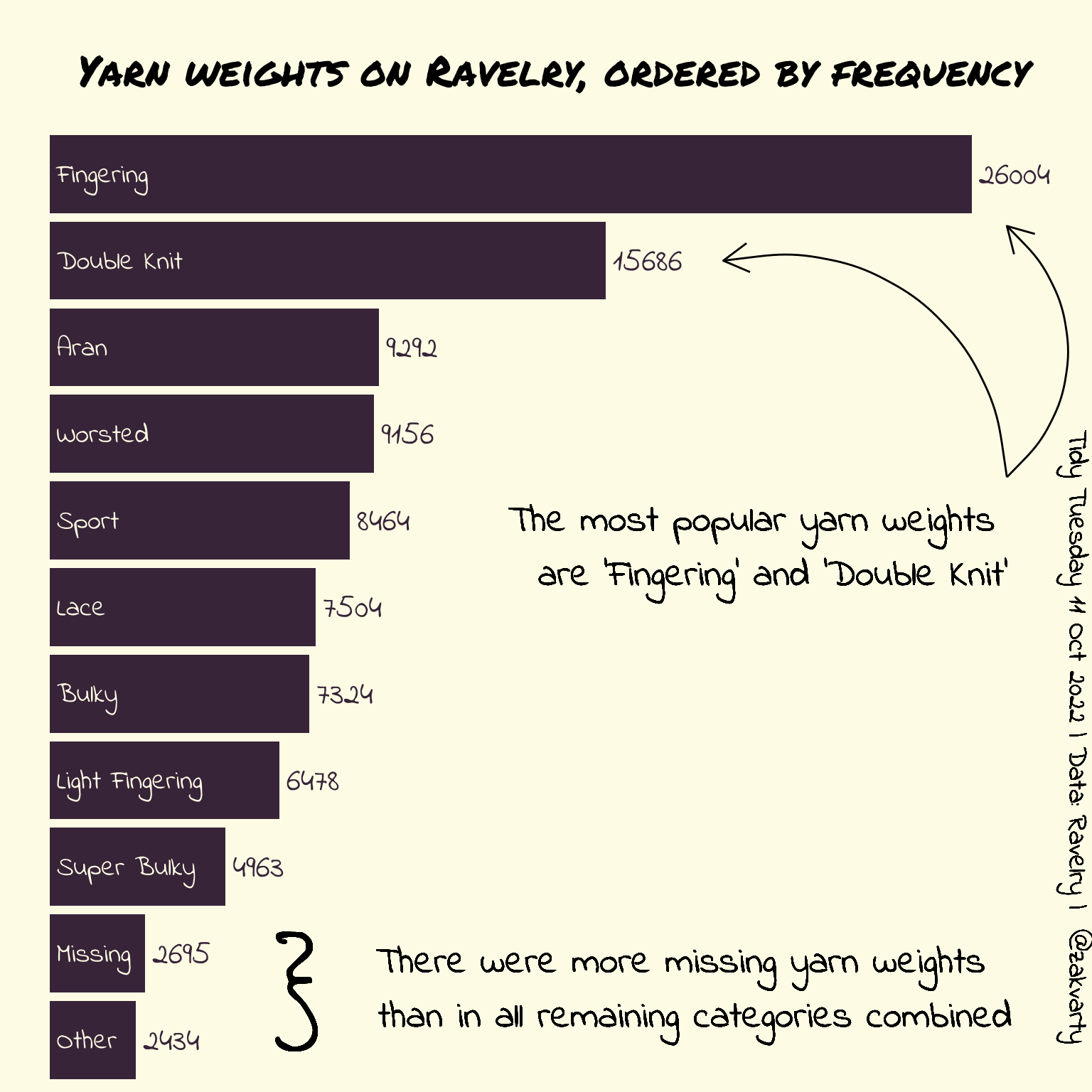
yarn_plot <- yarn_data %>%
  ggplot(aes(y = reorder(name, value), x = value)) +
  geom_bar(stat = "identity", fill = bar_colour) +
  theme_void() +
  ggtitle(" \n Yarn weights on Ravelry, ordered by frequency",subtitle = " ") +
  theme(axis.title = element_blank(),
        axis.text = element_blank(),
        axis.ticks = element_blank(),
        text = element_text(family = main_font),
        plot.background = element_rect(fill = bg_colour, colour = bg_colour),
        panel.background = element_rect(fill = bg_colour, colour = bg_colour),
        plot.title = element_text(family = title_font, size = 22, hjust = 0.5)
  ) +
  lims(x = c(0,28000)) +
  geom_text(aes(label = name, x = 200),
            color = bg_colour,
            hjust = 0,
            family = main_font,
            size = 5) +
  geom_text(aes(label = value),
            hjust = 0,
            nudge_x = 200,
            color = bar_colour,
            family = main_font,
            size = 6) +
  geom_text(aes(label = "The most popular yarn weights \n  are 'Fingering' and 'Double Knit'",
                x = 20000,
                y = 6.7),
            family = main_font,
            size = 7) +
  geom_text(aes(label = "There were more missing yarn weights \n than in all remaining categories combined",
                x = 18000,
                y = 1.6),
            family = main_font,
            size  = 7) +
  geom_text(aes(label = "}"),
            x = 7000,
            y = 1.5,
            size = 19,
            family = main_font) +
  geom_text(aes(label = "Tidy Tuesday 11 Oct 2022 | Data: Ravelry |  @zakvarty"),
            x = 29000,
            y = 4.5,
            size = 5,
            family = main_font,
            angle = 270) +
  geom_curve(aes(x = x1, y = y1, xend = x2, yend = y2),
             data = arrow_df_1,
             arrow = arrow(length = unit(0.03, "npc"))) +
  geom_curve(aes(x = x1, y = y1, xend = x2, yend = y2),
             data = arrow_df_2,
             arrow = arrow(length = unit(0.03, "npc")))

yarn_plot

# Exported as 8x8 inch pdf and 800x700 png
# (next time start by setting canvas size!)